
ART151 ART1674S
The tunnel diode, as the name suggests, is a diode, but with negative resistance characteristics that allow its use in circuits similar to relaxation oscillators with unijunction transistors or neon lamps. However, tunnel diodes have something more: they can oscillate at frequencies above 1 Gigahertz, which makes them especially suitable for very high frequency circuits.
Although tunnel diodes are not common components, the possibility of using these components in projects can be interesting when the main requirement is simplicity in very high frequency circuits.
HOW IT WORKS
Figure 1 shows the symbol commonly used to represent the tunnel diode.
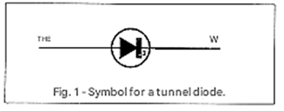
Its negative resistance properties come from the use of an ultra-thin depletion layer at the junction, which endows the component with negative resistance characteristics. The component's name comes from the fact that, unlike other semiconductors where the potential barrier resistance depends up to a certain value on the applied voltage, there is a point where these carriers find a kind of tunnel through which they can easily pass, resulting in a characteristic curve shown in Figure 2.
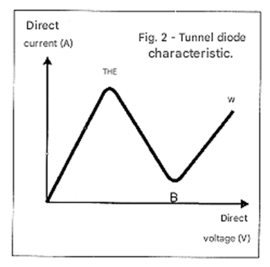
Thus, when a forward voltage is applied, the component behaves like a common diode until it reaches point A. This point occurs at a few tens of millivolts for common tunnel diodes and is called the "peak point". However, from this point onwards, when the voltage increases, instead of the current also increasing, it decreases abruptly until the so-called trough point shown in B.
In this section, we have an "abnormal" behavior for the component, which begins to exhibit negative resistance. Remember that the resistance in the graph in question is the cotangent of the angle that the characteristic curve presents at the point in question, and in this case, we have negative values for the section between A and B.
From point B onwards, the increase in voltage again causes an increase in current, at which point the component begins to exhibit behavior similar to other electronic components. However, the important aspect of the negative resistance characteristic that this component presents, which is similar to that of unijunction transistors and even neon lamps, is that the tunnel diode can be used in relaxation oscillators and even to amplify signals.
Because the action of tunnel diodes is extremely fast, unlike neon lamps and unijunction transistors whose operating speed limits their application to circuits of at most a few tens of kilohertz, tunnel diodes can be used in very high frequency circuits, easily exceeding 1000 MHz or 1 GHz. Some applications of tunnel diodes based on what we have seen are shown below:
VHF/UHF OSCILLATOR WITH TUNNEL DIODE
As we have seen, the negative resistance characteristics of the tunnel diode make this component ideal for use in oscillators. The circuit shown in Figure 3 is an example where, with the diode used, signals with frequencies up to 1.6 GHz can be generated.
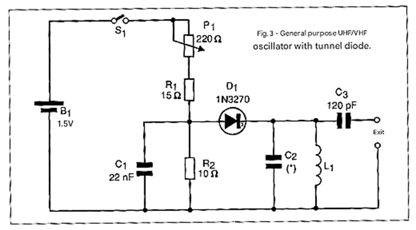
In fact, depending on the values of L1 and C2, which determine the circuit's frequency, we can make it oscillate in a range from a few kilohertz to over 1 GHz. For a coil formed by 2 turns of 22-gauge wire without a core, 0.5 cm in diameter, and a 2.2 pF capacitor, the oscillation frequencies can be between 100 and 200 MHz.
Note, however, that the tunnel point of diodes of this type occurs at a very low voltage; hence, the power supply is only 1.5 volts, and there is an adjustment made by P1 to find an intermediate point between the peak (A) and the valley (B) in the graph of Figure 2, which leads the circuit to oscillate with greater intensity. This is the only adjustment of this type of circuit and can be made with an oscilloscope connected to the oscillator output. Remember that the trimpot or adjustment potentiometer must be of the wire type. The capacitors must be ceramic, and the signal intensity is quite small, requiring amplification depending on the application.
CRYSTAL OSCILLATOR
The circuit shown in Figure 4 can generate frequencies ranging from a few hundred kilohertz to several Megahertz.
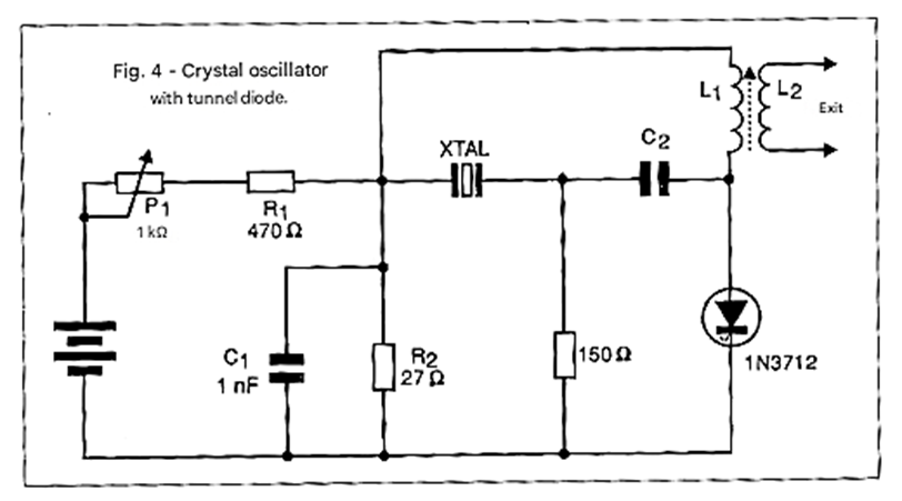
Capacitor C2, along with L1, must be calculated to form a resonant circuit at the crystal's frequency. Fine-tuning of this circuit to obtain maximum efficiency is done via the coil core. The signal is taken from L2, which consists of several turns on L1, according to the signal frequency. The operating point adjustment is done in the same way as in the previous circuit. The wire-wound potentiometer P1 must be set to a point where the voltage across the tunnel diode falls between points A and B on its characteristic curve, causing oscillation.
This adjustment can be easily done by connecting an oscilloscope to the signal input. Simply adjust P1 to obtain the signal with maximum intensity at the output and then fine-tune this adjustment on the coil core. In some cases, it may be necessary to switch the circuit on and off several times to get the oscillator to start during the adjustment process. Once adjusted for optimal performance, the possibility of failure to start will be minimized.
VOLTAGE-CONTROLLED RF OSCILLATOR
The circuit in Figure 5 generates signals between 7 and 15 MHz, with the frequency controlled by the input voltage according to the table of values given next to the diagram.
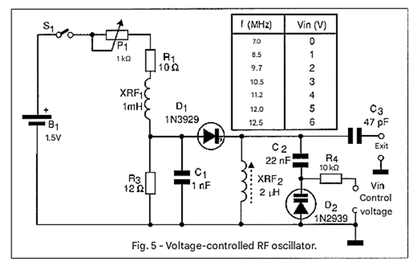
A variable capacitance diode (varicap) is used, and the values in the table are for the 1N2939 type. However, equivalents such as the BB109, BB809, or any other can be used; the reader should determine the new frequency range produced. An oscilloscope can be used for this purpose. XRF1 is an RF choke that should have an ohmic resistance no greater than 7 ohms. L1 has an inductance of 2 uH, or approximately 30 turns of 28-gauge wire on a ferrite rod 0.8 to 1 cm in diameter and 10 cm long. The capacitors should all be ceramic, and the adjustment procedures are similar to the two previous designs.
For the functional test and initial adjustments, the voltage at the control terminal can be zero. The control voltage range of this circuit depends on the varicap diode used.
SHORTWAVE CONVERTER
The simple circuit shown in Figure 6 converts shortwave signals between 3 MHz and 30 MHz into medium wave signals that can be noticed a common 550 to 1600 kHz receiver.
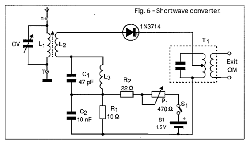
Tuning is done using CV, which together with L1 must cover the desired frequency range. For the 3 to 7 MHz range, for example, wind 30 turns of 28-gauge wire on a 10 cm ferrite rod and then add 10 turns on top of it to form L2. For the 7 to 15 MHz range, wind 15 turns of 28-gauge wire on a 10 cm ferrite rod and then add 5 turns on top of this coil to form L2. For the 15 to 30 MHz range, wind 12 turns.
The capacitor CV can be any variable capacitor from medium or shortwave radios with a maximum capacitance in the range of 180 to 300 pF. The maximum value of the capacitor used will determine the range covered by each coil. The reader should experiment by changing the number of turns in the coil according to the range to be covered and the capacitor used.
L3 together with capacitor C1 form the local oscillator. This coil can be similar to L1 for various bands and can eventually be modified to cover the desired bands. T1 is an AM radio oscillator coil that should be adjusted to around 1200 kHz or a free frequency in the medium wave band to which the radio should be tuned.
The adjustment should initially be made so that the circuit oscillates, which is achieved through P1 and using an oscilloscope or other means. Then CV and the core of T1 are adjusted to obtain the tuning of the desired bands. Eventually, changes to coil L3 may be necessary, or the other section of the variable capacitor can be used for C1, in which case L3 must be adjustable.
REGENERATIVE RECEIVER
The interesting circuit presented in Figure 7 can tune stations in the range from 200 kHz to 30 MHz depending on the coil used.
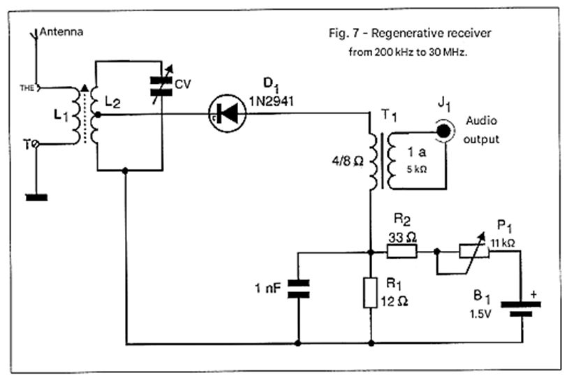
Obviously, given the low power of the output signal, a good audio amplifier should be used. We suggest a configuration with the LM386 or even the TDA2002 for a good experimental receiver. The coil should be wound according to the following table:
200 - 600 kHz –
L1 - 5 turns of 28 or 30 gauge wire over L2.
L2 - 220 turns of 28 to 30 gauge wire in a 1 cm diameter form with the tap on the 100th turn from the ground side.
600 to 1600 kHz –
L1 - 5 turns of 28 or 30 gauge wire over L2.
L2 - 100 turns of 28 or 30 gauge wire in a 1 cm diameter form with the tap on the 50th turn.
1600 to 3500 kHz –
L1 - 4 turns of 30 or 28 gauge wire over L2
L2 - 60 turns of 28 or 30 gauge wire in a 1 cm diameter loop with a tap on the 30th turn
3.5 to 9 MHz –
L1 - 4 turns of 28 or 30 gauge wire over L2
L2 - 25 turns of 28 or 30 gauge wire in a 1 cm diameter loop with a tap on the 12th turn
9 to 15 MHz –
L1 - 3 turns of 28 or 30 gauge wire over L2.
L2 - 11 turns of 28 or 30 gauge wire in a 1 cm diameter loop with a tap on the fifth turn.
15 to 30 MHz –
L1 - 2 turns of 28 or 30 gauge wire over L2
L2 - 6 turns of 28 or 30 gauge wire in a 1 cm diameter loop with a tap on the third turn
The form can be a coreless cardboard tube mounted on a 5-pin plug. The variable capacitor can have maximum capacitances between 180 and 360 pF. The capacitance range of the variable capacitor will determine the tuning range of the circuit, and there may be significant differences depending on these values, which can be compensated for by changing the number of turns in the coils. The values indicated above are for a variable capacitor with approximately a maximum capacitance of 360 pF.
The adjustment of the operation is done in the same way as explained in the previous projects. Transformer T1 can be a small output transformer found in old transistor radios.
TRANSMITTER
The transmitter shown in Figure 8 can be used for telegraphy training or as a short-range transmitter for a single-channel remote control system.
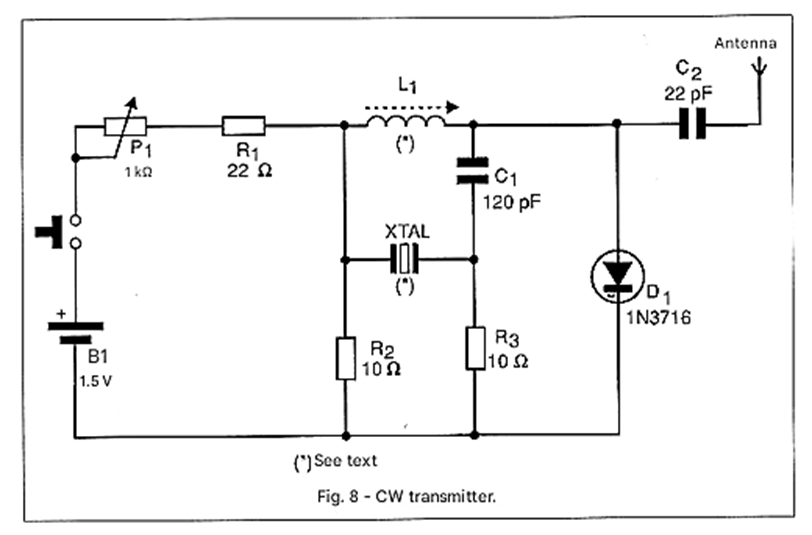
The L1 coil and C1 should resonate at the crystal's frequency. The L1 coil should be wound with wire that is not too thin so as not to present an ohmic resistance greater than about 5 ohms. For a crystal in the 27 MHz range, the L1 coil can have values between 0.2 and 0.4 uH, and the antenna is of the telescopic type. The operating point between points A and B of the tunnel diode's characteristic curve can be found by connecting an oscilloscope to the circuit's output.


